Rasters
All of these examples will start from the dem_4269.Tif raster in the demo dataset.
Start by adding dem_4269.tif to an empty project. Bonus points if you can tell me where it is... Elevation is in meters.
Terrain Processing
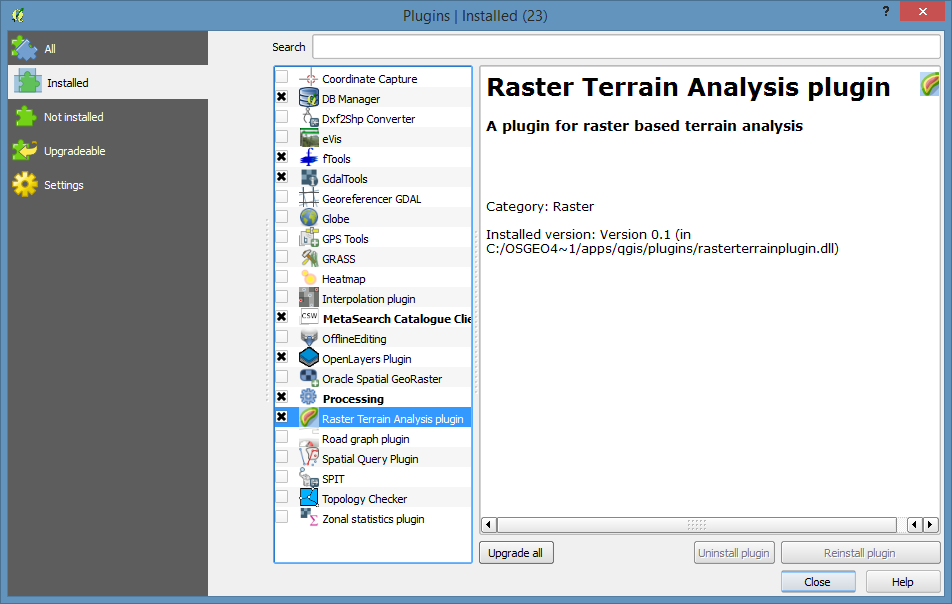
Add the Terrain Analysis Plugin
Go to Plugins, Manage and install plugins
Click on the Installed tab on the left. and look for the “Raster Terrain Analysis Plugin”, and turn it on with the check box to it’s left.
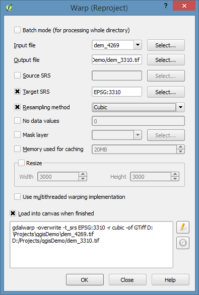
Reprojecting a Raster
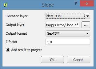
Reproject from the current geographic projection (NAD83) (EPSG: 4269) into something a little more friendly for doing terrain analysis (without using Z-factors).
Under the Raster menu, go to Projections and select Warp
I’m going to reproject it to California Albers NAD83 (EPSG: 3310) using the cubic convolution resampling method.
After the reprojection, I’m going to remove the 4269 dem, and set the project’s spatial reference to 3310. Set the spatial reference using the button at the lower right corner of QGIS.
Styling
By default many of the best color ramps for displaying terrain aren’t turned on.
To turn them on, we’ll use the Style Manager.
Open the Style Manager by going to the Settings manu, and selecting Style Manager
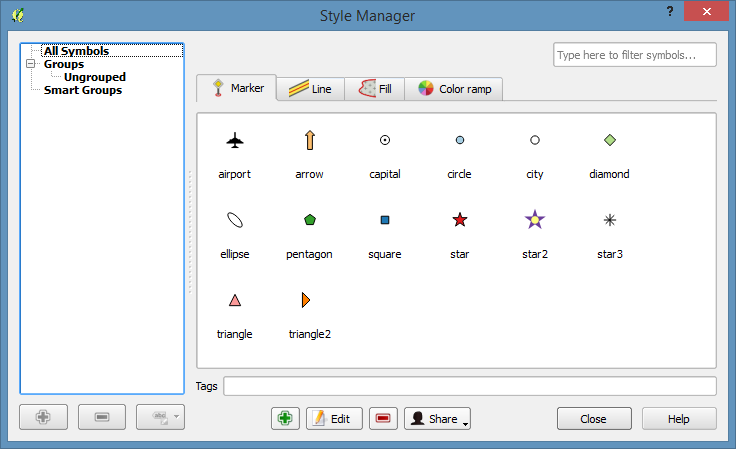
Then select the “Color Ramp” tab.
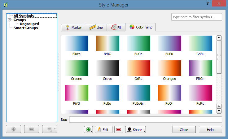
Click on the little green + sign to add a new style and select cpt-city
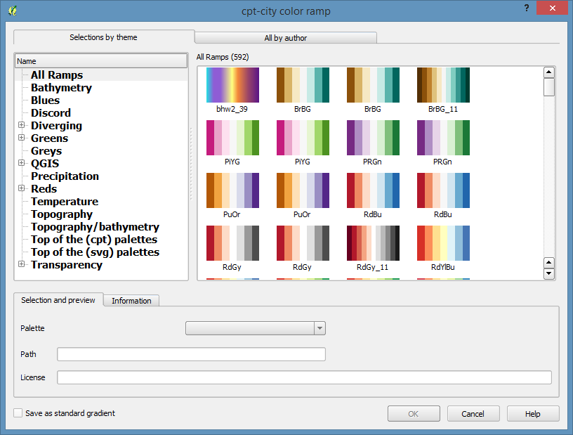
Then select the Topography section.
Scroll down to pick the wiki-schwartzwald-cont color ramp.
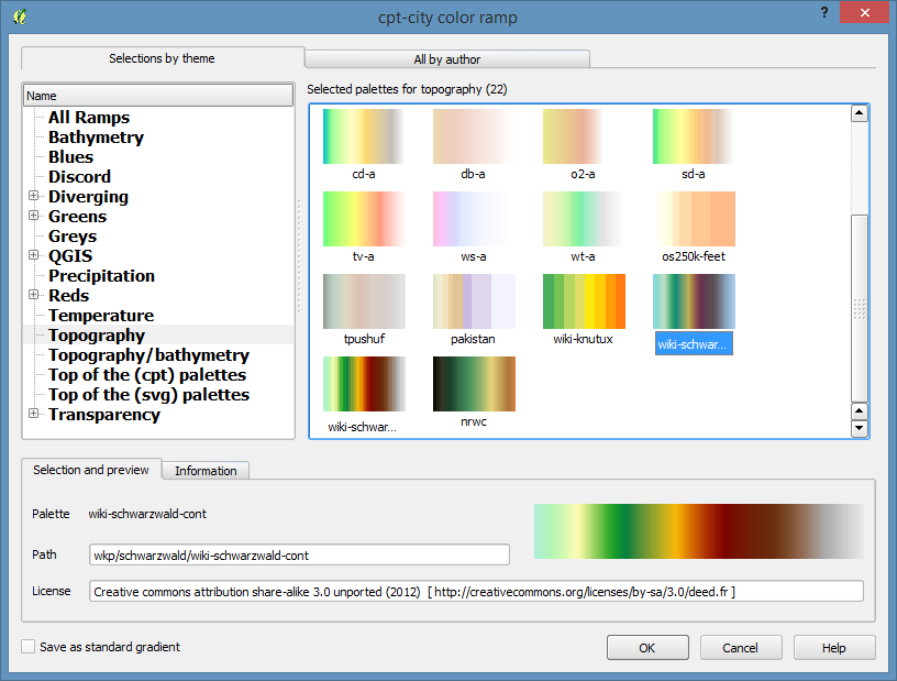
Then click OK and accept the default name for the gradient and close the style manager.
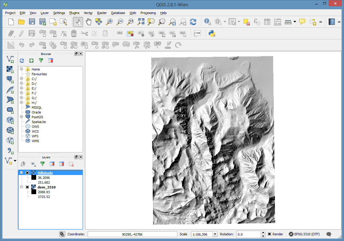
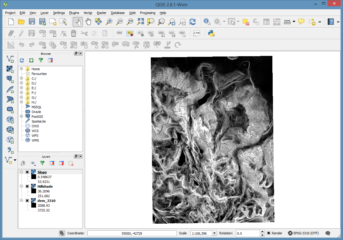
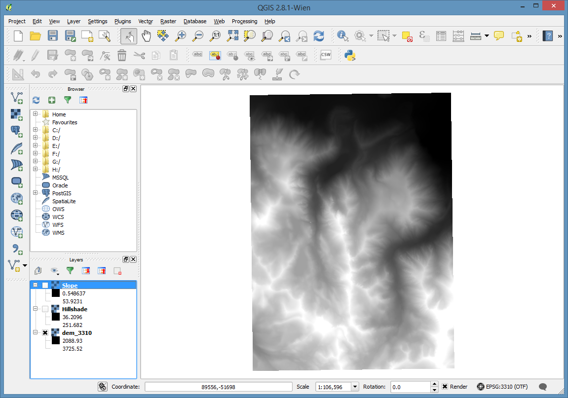
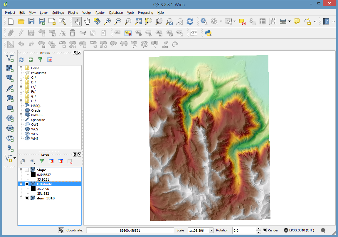
Last, let’s apply it to the dem.
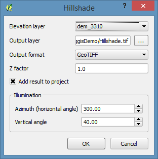
Turn off or reorder the layers so that the dem is visible. I suggest leaving the hillshade on top of the dem.
Double click on the dem layer and go to the layer’s Style properties page.
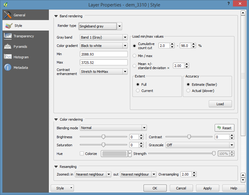
Set the Render type to Singleband pseudocolor, and under “Generate new color map” pick the wiki-schwartzwald-cont. Then click the Classify button.
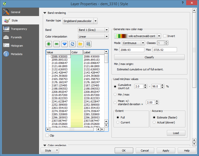
Now, Click OK
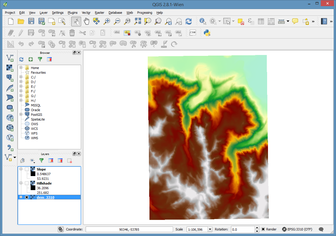
One last step. Let’s open the properties for the hillshade layer and go to the Transparancy settings. Set the transparancy to about 70%
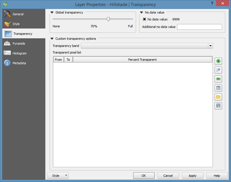
And click OK again. Then turn the layer on.
Raster Math
Reclassifying Datasets
First, we need to create some reclassified rasters from our existing DEM and Slope layers.
I’ve prepared some reclass text files to help us with this. Download these and put them in the same folder as your sample data.
Working through the Slope as an example. The DEM will work exactly the same way.
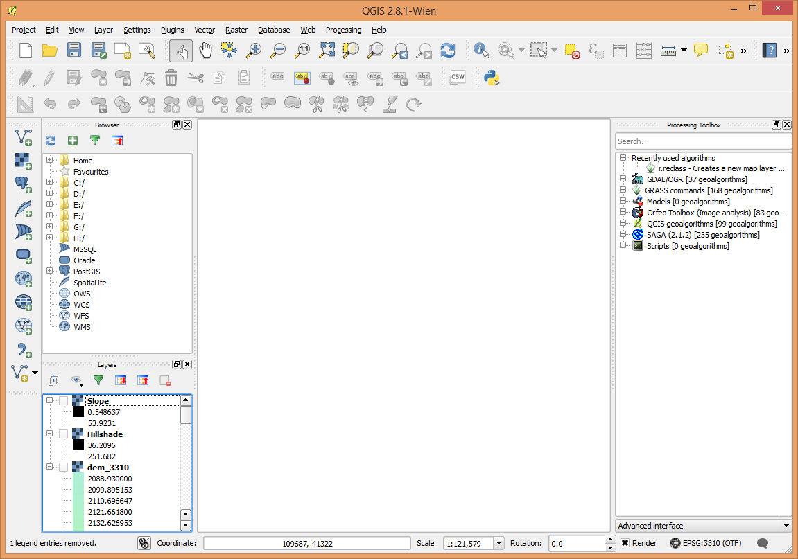
Open the Processing menu, and select Toolbox
Then at the bottom of the new window that opens select the Simple interface and switch it to Advanced interface.
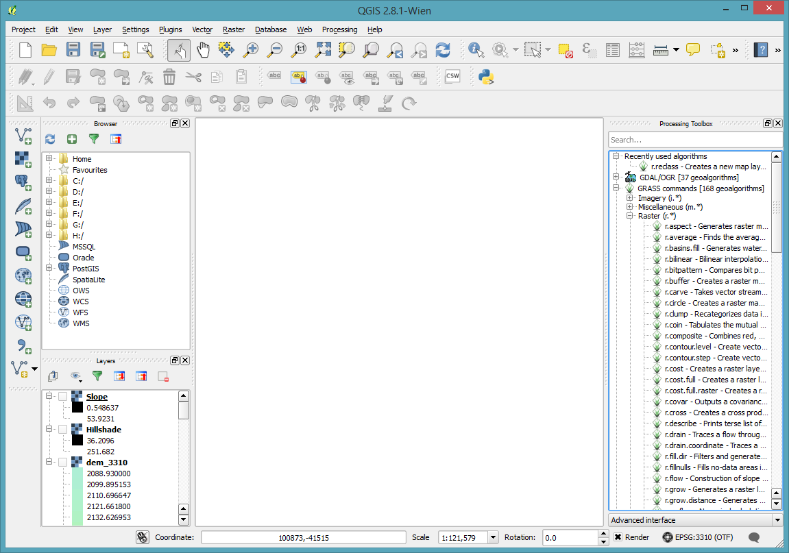
Open the GRASS commands, and the Raster (r.*) sections and navigate down to r.reclass
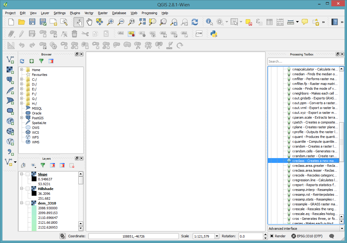
Double click on the tool to open the dialogue. Fill out the settings, making sure to select the correct input layer, reclass file, and set the output file.
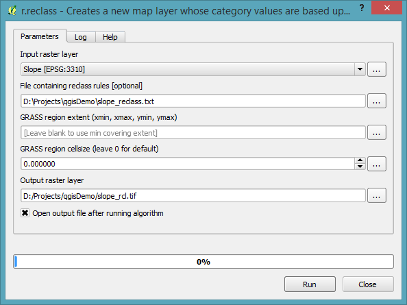
After clicking OK, the process will run and it will be added to the table of contents. Repeat the process for the DEM using the DEM’s reclass file.
For convenience, I’ve renamed the layers to the file name from the default that names that they have when added to the table of contents.
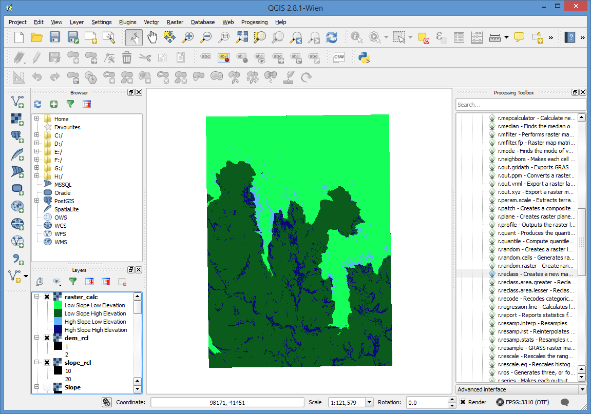
Raster Calculator
Map Algebra is then very simple.
Open the Raster menu and select Raster Calculator
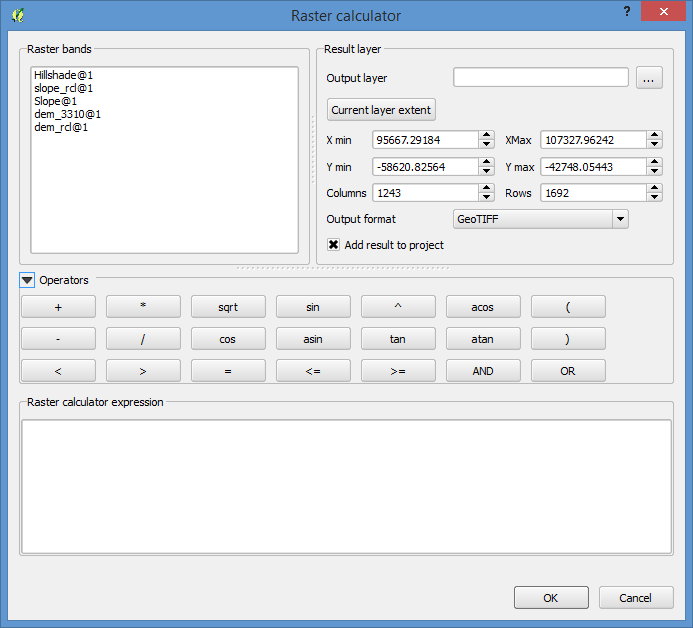
And build your map algebra function and set the output file.
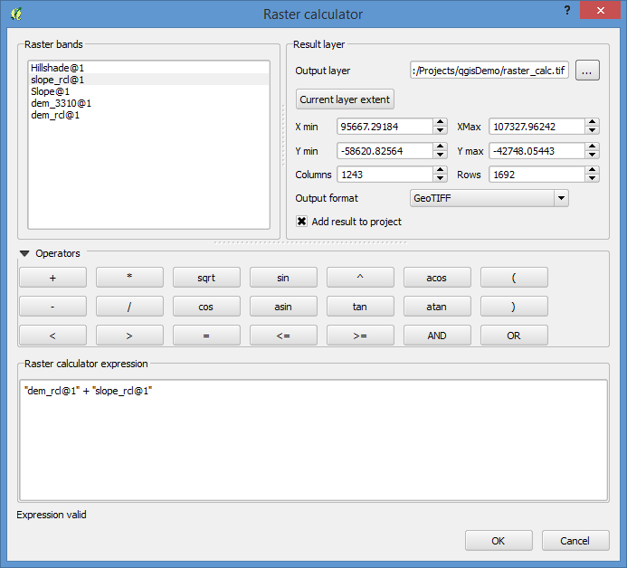
Then change the style on the layer to reflect the resulting classes. I used the Singleband pseudocolor renderer and added the values individually.
- 11: Low Slope, Low Elevation
- 12: Low Slope, High Elevation
- 21: High Slope, Low Elevation
- 22: High Slope, High Elevation